Pointing model run 2022/04
This new pointing model dataset was taken to replace the previous pointing model <Pointing-model-run-202111> using a new ATAOS look-up-table for the ATHexapod and ATPneumatics.
Observations
The data for this run was taken following a similar procedure to that of Observations.
A summary of the observations is shown in Observation journal.
| Night | Number of observations |
|---|---|
| 2022/04/07 | 53 |
Data Analysis
The data analysis follows a similar procedure to that of Data Analysis.
EFD Data Mining
papermill -p year 2022 -p month 04 -p day 06 -p time_window 4 -p efd_name summit_efd -p data_path /repo/LATISS reducing_pointing_data.ipynb reducing_pointing_data_2022_04_06_tw04.ipynb
Generating Pointing File
papermill -p pointing_data_file data/20220406/AT_point_data_20220406_tw004.pickle build_pointing_data.ipynb build_pointing_data_2022_04_06_tw04.ipynb
Generating Pointing Model
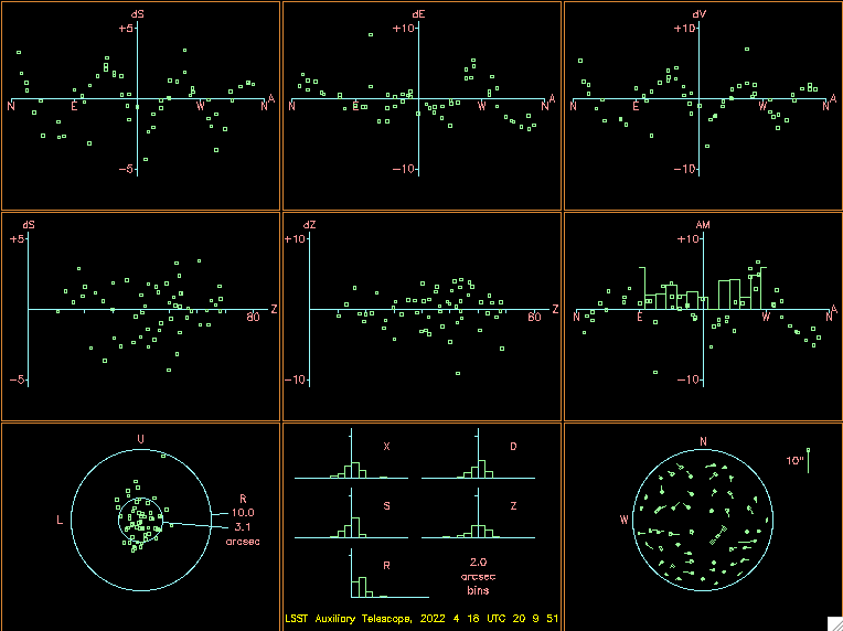
Fitting a simple 6-parameter pointing model to the data yields;
    coeff       change     value    sigma

1     IA         -6.821   -292.01    2.167
2     IE         +0.001   -213.05    0.909
3     AN         -0.005    +39.16    0.504
4     AW         +0.005    +70.89    0.498
5     TX10       +0.000     -6.86    0.723
6     CA        +10.214    +90.93    1.519

Sky RMS =   3.14
Popn SD =   3.33
fig-tpoint_a9plot_ia_ie_an_aw_tf_tx10_202204_tw004 below shows the diagnostics plots from this model.

The “9 favorite plots for altazimuth”. This plot gathers the 9 most relevant plots with information about the pointing model fit for an altaz mount.
Note that with respect to the previous pointing model <Pointing-model-run-202111>, we reduce the model to 6 parameters, instead of 7, and we still obtain better residues (3.14 arcsec rms instead of 4.45).
In the fitting process we usually start from the most simple coeffient, adding more complex one at each stage.
If the parameter value is smaller than the sigma value, we remove the coeffient from the fit.
In this case, the set of parameters that yield a good fit while still employing the most simple pointing coefficients is the one shown above.
Nevertheless, would also expect that we would end up with residues that does not show any correlated errors.
If you look at the top panels on fig-tpoint_a9plot_ia_ie_an_aw_tf_tx10_202204_tw004, you will notice that this is actually not the case and we still observe some correlated errors.
The top pannels refered above show the east-west residuals plotted against hour angle, the declination residuals plotted against declination and the Zenith-distance errors against zenith distance, from left-hand to right-hand respectively.
The correlated erros are more clear on the leftmost and rightmost plots.
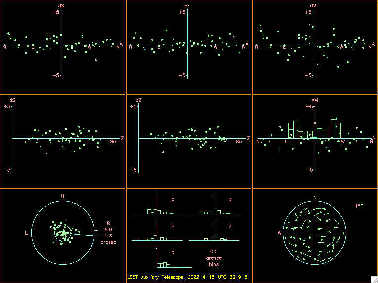
Since we were unable to remove these erros with a simple fit, we applied the automic fitting tool provided by tpoint. The result is;
And the diagnostics plots for this case is shown in fig-tpoint_a9plot_fauto_202204_tw004.

The “9 favorite plots for altazimuth”. This plot gathers the 9 most relevant plots with information about the pointing model fit for an altaz mount.
In this case, we observe a considerable improve in the fit residue (from 3.14 to 1.3 arcsec rms), though the number of coefficients jumps from 6 to 17 with the addition of several higher order coefficients.
We will have to explore how these two models perform on sky in order to decide which one is more suitable. We tend to preferr simpler models as they give better performance is regions not covered by pointing data, whereas higher order models can produce some undesirable extrapolation effects.